Welfare Maximizing Market Clearing

Welfare Maximizing Market Clearing#

Given the demand function and the bids from the producers we want to clear the market such that welfare is maximized. We define welfare as the difference between market value ($V$) and producer cost ($C$).

1. Load packages

We are using the gurobipy package to formulate a mathematical model and solve it.

import numpy as np
import gurobipy as gp
from gurobipy import GRB

import matplotlib.pyplot as plt

2. Define Parameters

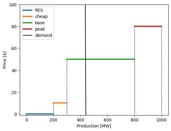
We study an exemplary market with 4 producers with the following offers:

Producer	Offer price in $/MW	Offer amount in MW
Renewable	0	2
Cheap	10	100
Base	50	500
Peak	80	20

We model demand through an inverse demand-price functon: $\pi(q^D) = \beta q^D + \pi^{max}$ with the following parameters:

$\beta= -25$
$\pi^{max} = 11,000$.

We first define these parameters and create a basic visualization.

# Inverse price demand function
# pi(q) = beta * q + pi_max
beta = -25
pi_max = 11e3
# We can use a lambda function to define this relationship in a single line
pi = lambda q: beta*q + pi_max

# Generators
c = [0, 10, 50, 80] # vector of cost [$/MW]
p_max = [200, 100, 500, 200] # vector of maximum capacity [MW]
gen_type = ["RES", "cheap", "base", "peak"]
n_gen = len(c) # number of generators

# Create a vizualization

# First plot the individual offer bids
fig, ax = plt.subplots(1,1)
# The subplots(x,y) command creates a figure with x rows and y columns of plots.
# Here we only want one plot. Using subplots(1,2) would create two plots next to each other inside the same figure.

# Each bid is essentially a horizontal line that we can define through its start and end point
for i in range(n_gen):
  x1 = sum(p_max[:i]) # define the start point of each line
  x2 = sum(p_max[:i+1]) # define the end point of each line
  x = [x1, x2]
  y = [c[i], c[i]]
  ax.plot(x, y, label=gen_type[i], linewidth=3) # plot the line

  # At vertical lines to make it nice
  ax.vlines([x1, x2], 0, c[i], 'black', 'dashed', linewidth=0.8)


# Now lets add the demand function by creating some points
xs = np.arange(0, 1000, 50) # creates a list of number from 0 to 1000 in steps of 50
ys = [pi(x) for x in xs] # creates a list of resulting prices using "list comprehension"

# Plot the line
ax.plot(xs, ys, 'black', label="demand")

# Enable legend
ax.legend() # turn legend on

# Add axis labels
ax.set_ylabel("Price [$]")
ax.set_xlabel("Production [MW]")

# Restrict the visible plot to the relevant area
ax.set_ylim([-1, 100]);

../_images/7a53447512e3d5d96b95613600bf125e5310b4a3509f4b21621e89b930e60920.png

3. Define mathematical model

Let $\pi^*$ be the market price and $q^*$ the market quantity after clearing. From this we get:

(4)#\[\begin{align} V &= \frac{1}{2}q^*(\pi^{max} - \pi^*) + q^*\pi^* = \frac{1}{2}q^*(\pi^* + \pi^{max}) = \frac{1}{2}q^*(\beta q^* + \pi^{max} + \pi^{max}) \\ &= \frac{1}{2} \beta (q^*)^2 + \pi^{max}q^* \\ C &= \sum_{i=1}^G c_i q_i^{G,*} \end{align}\]

So the resulting market clearing problem is:

(5)#\[\begin{align} \max_{q^G, q^D} \quad &V - C \\ \text{s.t.} \quad & \sum_{i=1}^G c_i q_i^{G} = q^D \\ & q_i^G \le q_i^{G,max} \quad i \in [G] \\ & q_i^G, q^D \ge 0 \end{align}\]

# define the optimization program

m = gp.Model()
m.setParam('OutputFlag', 0)

# variables
p = m.addVars(n_gen, lb=0, ub=GRB.INFINITY, name="p")
d = m.addVar(lb=0, ub=GRB.INFINITY, name="d")

# constraints
m.addConstr(p.sum() == d, name="enerbal")
for i in range(n_gen):
    m.addConstr(p[i] <= p_max[i])

# define objective
V = 0.5*beta*(d**2) + pi_max*d
C = sum(p[i]*c[i] for i in range(n_gen))
welfare = V - C
m.setObjective(welfare, GRB.MAXIMIZE)

Set parameter Username

Academic license - for non-commercial use only - expires 2025-11-15

# clear the market and print the results
m.optimize()

welfare_res = m.ObjVal
d_res = d.X
p_res = [p[i].X for i in range(n_gen)]
C_res = C.getValue()
print(f"Resulting welfare: {welfare_res:.1f} $")
print(f"Resulting generation cost: {C_res:.1f} $")
print(f"Resulting demand:  {d_res:.1f} MW")
print(f"Generator outputs:")
for i in range(n_gen):
  print(f"   {gen_type[i]}: {p_res[i]:.1f} MW")

Resulting welfare: 2412050.0 $
Resulting generation cost: 7900.0 $
Resulting demand:  438.0 MW
Generator outputs:
   RES: 200.0 MW
   cheap: 100.0 MW
   base: 138.0 MW
   peak: 0.0 MW

# compute the price
pi_opt = pi(d_res)
print(f"The market clearing price is {pi_opt:.1f} $/MW")

The market clearing price is 50.0 $/MW

# compute the dual of the energy balance

lam = m.getConstrByName("enerbal").Pi
print(f"The dual of the energy balance is {lam:.1f}")

The dual of the energy balance is -50.0

# let's redo the computation as our known ED with fixed demand

D = d_res

m = gp.Model()
m.setParam('OutputFlag', 0)

# variables
p = m.addVars(n_gen, lb=0, ub=GRB.INFINITY, name="p")

# constraints
m.addConstr(p.sum() == D, name="enerbal")
for i in range(n_gen):
    m.addConstr(p[i] <= p_max[i])

# define objective
C = sum(p[i]*c[i] for i in range(n_gen))
m.setObjective(C, GRB.MINIMIZE)

# clear the market and print the results
m.optimize()

welfare_res = m.ObjVal
p_res = [m.getVarByName(f"p[{i}]").X for i in range(n_gen)]
C_res = C.getValue()
print(f"Resulting welfare: {welfare_res:.1f} $")
print(f"Resulting generation cost: {C_res:.1f} $")
print(f"Resulting demand:  {d_res:.1f} MW")
print(f"Generator outputs:")
for i in range(n_gen):
  print(f"   {gen_type[i]}: {p_res[i]:.1f} MW")

print()
lam = m.getConstrByName("enerbal").Pi
print(f"The dual of the energy balance is {lam:.1f}")

Resulting welfare: 7900.0 $
Resulting generation cost: 7900.0 $
Resulting demand:  438.0 MW
Generator outputs:
   RES: 200.0 MW
   cheap: 100.0 MW
   base: 138.0 MW
   peak: 0.0 MW

The dual of the energy balance is 50.0