Economic Dispatch

Economic dispatch is the process of deciding the most optimal economic dispatch strategy from a given generator portfolio to reliably meet power demand (load).

1. Load packages and useful definitions

• We are using the gurobipy package to formulate a mathematical model and solve it.

# import required packages

import pandas as pd
import numpy as np

import gurobipy as gp
from gurobipy import GRB

import matplotlib.pyplot as plt

# some helpful definitions

gen_colors = {
    "Hydro": "#1f78b4",  # Deep Blue
    "Nuclear": "#e31a1c",  # Red
    "Coal": "#8b4513",  # Dark Brown
    "Gas CC": "#8e44ad",  # Medium Purple
    "Gas CT": "#a569bd",  # Light Purple
    "Oil CT": "#4d4d4d",  # Dark Gray
    "Wind": "#6baed6",  # Light Sky Blue
    "PV": "#ff7f00"  # Bright Orange
}

def print_gp_status(m):
    status = m.Status
    if status == GRB.OPTIMAL:
        print("The model is optimal.")
    elif status == GRB.INFEASIBLE:
        print("The model is infeasible.")
    elif status == GRB.UNBOUNDED:
        print("The model is unbounded.")
    else:
        print(f"Optimization ended with status {status}.")
    print()
    return status

2. Read and prepare data

• The data is simplified generator data. We have entries for each type of generator (not generator unit specific).

• It includes cost data, fixed cost and variable cost. It also includes technical limitations like the installed amount, minimum generation levels, ramping rates, minimum down time and minimum up time (minimum run time).

# read the data
data_file = "ts_and_gen.xlsx"
load_and_res_data = pd.read_excel(data_file, sheet_name=0)
gen_data = pd.read_excel(data_file, sheet_name=1)

# inspect the data
gen_data

	Unit Type	Fixed Cost USD/kW	Variable Cost USD/MWh	Installed in MW	PMin in MW	Ramp Rate in MW /hr	Min Down Time Hr	Min Up Time Hr
0	Nuclear	8000	3	3000	2650	300	48	24
1	Oil CT	1200	50	2000	400	1500	1	1
2	Coal	3000	10	5000	1750	2000	10	10
3	Hydro	3000	2	3000	0	3000	0	0
4	Gas CC	1000	25	15000	7500	2500	4	8
5	Gas CT	800	35	3000	600	9000	2	2

# prepare data for economic dispatch

# generator data
gen_type = gen_data['Unit Type'].to_numpy()
mc = gen_data['Variable Cost USD/MWh'].to_numpy()
Pmax = gen_data['Installed in MW'].to_numpy()
R60 = gen_data['Ramp Rate in MW /hr'].to_numpy()
n_gen = len(gen_type)

# load data
load = load_and_res_data['CAISO (MW)'].to_numpy()
n_t = len(load)

# Res data
wind = load_and_res_data['10 000 MW Onshore Wind'].to_numpy()
pv = load_and_res_data['15 000 MW Solar PV'].to_numpy()
curt_pen = 0 # $/MWh

3. Inspect data

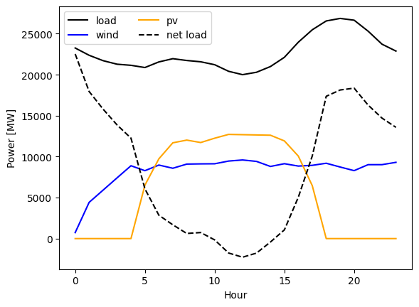
• We can see the very typical duck curve (area between load and net-load looks like a duck). The net load is the load subtracted by RES production (in this case Wind and PV).

fig, ax = plt.subplots(1,1)
ax.plot(load, label="load", color="black")
ax.plot(wind, label="wind", color="blue")
ax.plot(pv, label="pv", color="orange")
ax.plot(load-wind-pv, label="net load", color="black", ls="--")
ax.set_ylabel("Power [MW]")
ax.set_xlabel("Hour")
ax.legend(ncols=2);

4. Define mathematical model We implement the following economic dispatch with renewable energy generation (RES).

Objective function:

• Minimize the sum of cost of generation \(C_t^{\text{gen}}\) and curtailment \(C_t^{\text{curt}}\) over time T.

Decision variables:

• \(p_{i,t}^{\text{c}}\) production of conventional generator i in t.

• \(p_{i,t}^{\text{w}}\) production of wind generator i in t.

• \(p_{i,t}^{\text{pv}}\) production of PV i in t.

Constraints:

• Generation cost \(C_t^{\text{gen}}\) is equal to the cost function \(c_i(p^{\text{c}}_{i,t})\)

• Curtailment cost \(C_t^{\text{curt}}\) is equal to the difference between the RES production limit \(\overline{P}_{i,t}^{\text{w}}\), \(\overline{P}_{i,t}^{\text{pv}}\) and the realized production of RES \(p_{i,t}^{\text{w}}\), \(p_{i,t}^{\text{pv}}\).

• The sum of generation needs to equal the demand \(D_t\) in each t.

• Generator output needs to be greater or equal to 0 and smaller or equal to their respective production limits, which are time-dependent t for RES.

• Conventional generators have ramping constraints, which limits how much their generation \(p_{i,t}^{\text{c}}\) can change up or down from one time step to the next. It is limit by \(R_i^{\text{60}}\).

(3)\[\begin{align} \min \quad & \sum_{t=1}^T C_t^{\text{gen}} + C_t^{\text{curt}} \\ \text{s.t.} \quad & C_t^{\text{gen}} = \sum_{i \in [G]} c_i(p^{\text{c}}_{i,t}) && \forall t \in [T] \\ & C_t^{\text{curt}} = c^{\text{curt}} \Big[ \sum_{i \in W} (\overline{P}_{i,t}^{\text{w}} - p_{i,t}^{\text{w}}) + \sum_{i \in [PV]} (\overline{P}_{i,t}^{\text{pv}} - p_{i,t}^{\text{pv}}) \Big] && \forall t \in [T] \\ & \sum_{i \in [G]} p_{i,t}^{\text{c}} + \sum_{i \in [W]} p_{i,t}^{\text{w}} + \sum_{i \in [PV]} p_{i,t}^{\text{pv}} = D_t && \forall t \in [T] \\ & 0 \leq p_{i,t}^{\text{c}} \leq \overline{P}_{i} && \forall i \in [G] \\ & 0 \leq p_{i,t}^{\diamond} \leq \overline{P}_{i,t}, \quad \diamond=\{\text{w, pv}\} && \forall i \in [G] , t \in [T] \\ & |p_{i,t}^{\text{c}} - p_{i,t-1}^{\text{c}} | \leq R_i^{\text{60}} && \forall i \in [G], t \in [T] \end{align}\]

# write the ED model
m = gp.Model()
m.setParam("OutputFlag", 0)

# add variables
p = m.addVars(n_gen, n_t, lb=0, ub=GRB.INFINITY, name="p")
p_wind = m.addVars(n_t, lb=0, ub=GRB.INFINITY, name="p_wind")
p_pv = m.addVars(n_t, lb=0, ub=GRB.INFINITY, name="p_pv")

# energy balance
m.addConstrs((sum(p[i,t] for i in range(n_gen)) + p_wind[t] + p_pv[t] == load[t] for t in range(n_t)), name="energy_balance")

# generator constraints
for t in range(n_t):
    for i in range(n_gen):
        # maximum generation
        m.addConstr(p[i,t] <= Pmax[i])
        # ramping
        if t>0:
            m.addConstr(p[i,t] - p[i,t-1] <= R60[i])
            m.addConstr(p[i,t-1] - p[i,t] <= R60[i])

# RES constraints
for t in range(n_t):
    m.addConstr(p_wind[t] <= wind[t])
    m.addConstr(p_pv[t] <= pv[t])
        
# objective
gen_cost = sum(sum(mc[i]*p[i,t] for i in range(n_gen)) for t in range(n_t))
curt_cost = sum(curt_pen* ((pv[t]-p_pv[t]) + (wind[t]-p_wind[t])) for t in range(n_t))
m.setObjective(
    gen_cost + curt_cost, GRB.MINIMIZE
)

# run
m.optimize()

Set parameter Username

Academic license - for non-commercial use only - expires 2025-11-15

5. Inspect the solution and plot the dispatch

# Check the status of the solver
print_gp_status(m)

# Objective value
objective = m.ObjVal
print(f"Objective value {objective/1e6:.3f} M$.\n")

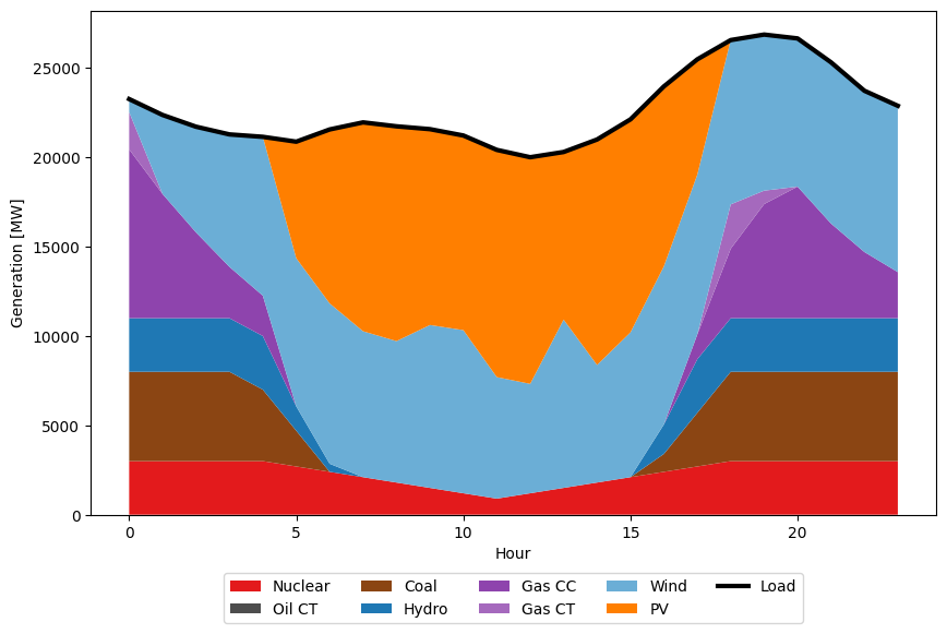
# prodcution plot
p_res = {type: [m.getVarByName(f"p[{i},{t}]").X for t in range(n_t)] for (i,type) in enumerate(gen_type)}
p_res['Wind'] = [m.getVarByName(f"p_wind[{t}]").X for t in range(n_t)]
p_res['PV'] = [m.getVarByName(f"p_pv[{t}]").X for t in range(n_t)]

#curtailment
wind_curt_res = wind - np.array(p_res['Wind'])
pv_curt_res = pv - np.array(p_res['PV'])
print(f"A total of {sum(wind_curt_res):.2f} MWh wind were curtailed.")
print(f"A total of {sum(pv_curt_res):.2f} MWh PV were curtailed.")

# plot
fig, ax = plt.subplots(1,1)
fig.set_size_inches(10,6)
x = np.arange(24)
color_list = [gen_colors[g] for g in list(p_res.keys())]
ax.stackplot(x, list(p_res.values()), labels=list(p_res.keys()), colors=color_list);
ax.plot(load, linewidth=3, color='black', label='Load')
ax.set_xlabel("Hour")
ax.set_ylabel("Generation [MW]")
ax.legend(ncols=5, loc="lower center", bbox_to_anchor=(0.5, -0.23));

The model is optimal.

Objective value 2.460 M$.

A total of 10980.62 MWh wind were curtailed.
A total of 5392.55 MWh PV were curtailed.